Introduction
This is a project maintained by myself, Indraneil Paul and co-contributor, Soham Saha that interprets a large number of Computer Science research papers from the DBLP archives and using the availble set of tags corresponding to each paper from an array of third-party sources, tries to predict a field in which a certain author is likely to contribute in the near-future.
Hosted here is a snapshot and brief discussion of the various challenges we faced and the ways that we tackled them.
Data Wrangling and Mapping
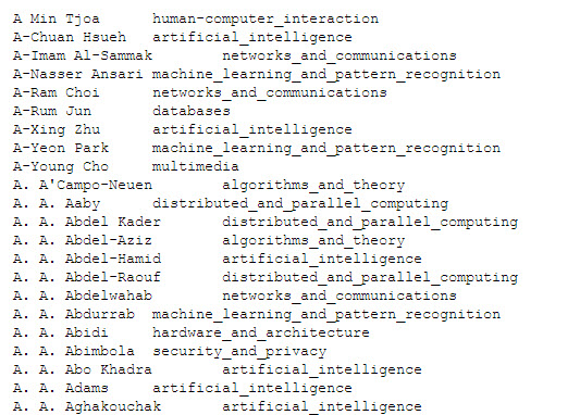
The original DBLP dump consisted of 294,000+ authors but their fields of work were not clearly mentioned. Using the previously done work of third party sources, tag information regarding the field of work of a large number of authors was found, andd then by matching the two sources we were able to salvage the tag information of as many as 216,000+ authors. A segment of the mapping has been shown below.
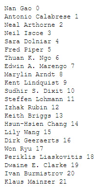
The groundwork for the later learning, by negative sampling using a skip-gram model was also laid at this phase, with an author to authorID mapping created and the negative sampling tuples also written to a context file in the form AuthorID1,AuthorID2,AuthorID3 where AuthorID1 and AuthorID2 could be two of the many authors who had collaborated on a paper. For each pair of authors, three different random negative samples were used in the form of three different AuthorID3 which indicated three authors the collaborating pair had not co-collborated with. A segment of the context has been shown below.
Author2Vec and Negative Sampling
The next phase of our project invovlved the formulation of context vectors for each author using the skip-gram model as with the context file elaborated above, as input.
####Motivation for using word vectors
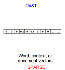
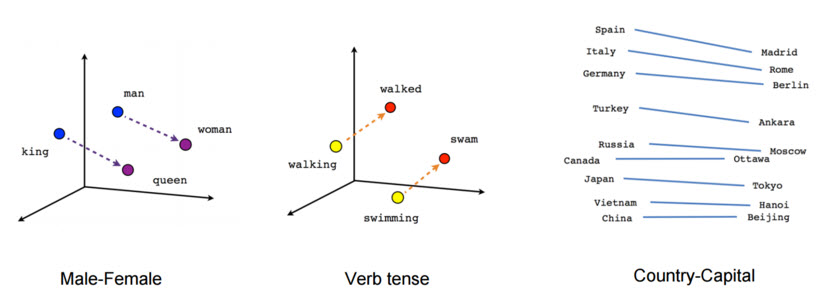
Natural language processing systems traditionally treat words as discrete atomic symbols, and therefore ‘cat’ may be represented as Id537 and ‘dog’ as Id143. These encodings are arbitrary, and provide no useful information to the system regarding the relationships that may exist between the individual symbols. This means that the model can leverage very little of what it has learned about ‘cats’ when it is processing data about ‘dogs’ (such that they are both animals, four-legged, pets, etc.). Representing words as unique, discrete ids furthermore leads to data sparsity, and usually means that we may need more data in order to successfully train statistical models. Using vector representations can overcome some of these obstacles. Vector space models (VSMs) represent (embed) words in a continuous vector space where semantically similar words are mapped to nearby points (‘are embedded nearby each other’).
Word2vec is a particularly computationally-efficient predictive model for learning word embeddings from raw text. It comes in two flavors, the Continuous Bag-of-Words model (CBOW) and the Skip-Gram model. Algorithmically, these models are similar, except that CBOW predicts target words (e.g. ‘mat’) from source context words (‘the cat sits on the’), while the skip-gram does the inverse and predicts source context-words from the target words.
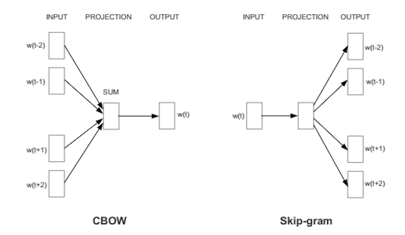
This inversion might seem like an arbitrary choice, but statistically it has the effect that CBOW smoothes over a lot of the distributional information (by treating an entire context as one observation). For the most part, this turns out to be a useful thing for smaller datasets. However, skip-gram treats each context-target pair as a new observation, and this tends to do better when we have larger datasets, which is why we went forward with it.
####Skip-Gram Model
Let’s imagine at training step t we observe the first training case above, where the goal is to predict the from quick. We select num_noise number of noisy (contrastive) examples by drawing from some noise distribution, typically the unigram distribution, P(w). For simplicity let’s say num_noise=1 and we select sheep as a noisy example. Next we compute the loss for this pair of observed and noisy examples. The goal is to make an update to the embedding parameters θ to improve (in this case, maximize) this objective function.

We do this by deriving the gradient of the loss with respect to the embedding parameters θ. We then perform an update to the embeddings by taking a small step in the direction of the gradient.
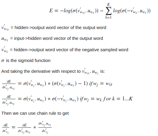
When this process is repeated over the entire training set, this has the effect of ‘moving’ the embedding vectors around for each word until the model is successful at discriminating real words from noise words.
Effectively, SKip Gram Negative Sampling is implicitly factorizing a word-context matrix, whose cells are the pointwise mutual information (PMI) of the respective word and context pairs, shifted by a global constant.
####Transfer Function
We took to the frequently-used sigmoid module as the trandfer function. This module applies the Sigmoid function element-wise to the input Tensor, thus outputting a Tensor of the same dimension. Sigmoid is defined as f(x) = 1/(1+exp(-x)).
####Loss Function Criteria In this project we have used the Binary Cross Entropy Criterion which creates a criterion that measures the Binary Cross Entropy between the target and the output.
criterion = nn.BCECriterion([weights])
This is used for measuring the error of a reconstruction in for example an auto-encoder. Note that the targets t[i] should be numbers between 0 and 1, for instance, the output of an nn.Sigmoid layer.
loss(o, t) = - 1/n sum_i (t[i] * log(o[i]) + (1 - t[i]) * log(1 - o[i]))
By default, the losses are averaged for each minibatch over observations as well as over dimensions. However, if the field sizeAverage is set to false, the losses are instead summed.
Transaction Speedup and Efficiency
The sheer size of the dataset was a challenge in itself. Runnning on subsets of over 40,000 authors proved to be infeasably slow and thus prompted us to look for other alternatives, as we needed to perform the task on a sample six times larger.
Also we needed a solution to the slew of memory-errors that we were frequently experiencing and as a result, we turned to the lmdb.torch plugin. This was essentially a wrapper for the lightningmdb plugin for torch which was an extremely efficient implementation of the memory-mapped database. The Lightning Memory-Mapped Database (LMDB) is a software library that provides a high-performance embedded transactional database in the form of a key-value store. LMDB is written in C with API bindings for several programming languages such as torch on lua. LMDB stores arbitrary key/data pairs as byte arrays, has a range-based search capability, supports multiple data items for a single key and has a special mode for appending records at the end of the database which gives a dramatic write performance increase over other similar stores.
Some attractive features of LMDB, that prompted us to use it in our project, include:
- Its use of B+Tree. With an LMDB instance being in shared memory and the B+Tree block size being set to the OS page size, access to an LMDB store is extremely memory efficient.
- As LMDB is memory-mapped, it can return direct pointers to memory addresses of keys and values through its API, thereby avoiding unnecessary and expensive copying of memory. This results in greatly-increased performance (especially when the values stored are extremely large), and expands the potential use cases for LMDB.
- LMDB also tracks unused memory pages, using a B+Tree to keep track of pages freed (no longer needed) during transactions. By tracking unused pages the need for garbage-collection (and a garbage collection phase which would consume CPU cycles) is completely avoided.
Also to the end of improving code efficiency, we used a lua library called lds which implements fast an efficient data structures. The lds library provides the containers Array, Vector, and HashMap, which cover the common use cases of Lua tables. However, the memory of these containers are managed through user-specified allocators (e.g. malloc) and thus are not subject to the LuaJIT memory limit. It is also significantly lower load on the LuaJIT Garbage Collector.
Classification
In the final phase an author was to be categorized into one of the fields in which he was most likely to work on in the near future. There were 25 such classes such as Artificial Intelligence, Computational Biology, etc which were assigned unique labels ranging from 0 to 24.
Subsequentlty, a technique of classification was to be chosen. Here we chose to use Support Vector Machine(SVM) to learn the classification boundaries, using the python library scikit-learn. Our choice of SVM as the technique of classification was influenced by the following factors:
- Effective in high dimensional spaces. This was crucial to us since the embedding size of the vectors learnt for each author was a 100.
- Still effective in cases where number of dimensions is greater than the number of samples.
- Uses a subset of training points in the decision function (called support vectors), so it is also memory efficient. Again, vital to us as we had an enormous archive dump to train and test upon.
- Versatile as different Kernel functions can be specified for the decision function.
Results
The scikit-learn package allows for two separate strategies to tackle multi-class classification problems using SVM, by providing the SVC, the NuSVC and the Linear SVC classes. Briefly discussed, they are:
- The “One-vs-One Strategy”:
SVCandNuSVCimplement the “one-against-one” approach (Knerr et al., 1990) for multi- class classification. Ifn_classis the number of classes, thenn_class * (n_class - 1) / 2classifiers are constructed and each one trains data from two classes. - The “One-vs-All Strategy”: The
LinearSVCimplements “one-vs-the-rest” multi-class strategy, thus trainingn_classmodels. If there are only two classes, only one model is trained. - Crammer and Singer Method: This is a multiclass SVM method which casts the multiclass classification problem into a single optimization problem, rather than decomposing it into multiple binary classification problems. The
LinearSVCclass implements this uding themulti_class='crammer_singer'option. This method is consistent, which is not true for one-vs-rest classification. In practice, one-vs-rest classification is usually preferred, since the results are mostly similar, but the runtime is significantly less.
The SVC and NuSVC are similar methods, but accept slightly different sets of parameters and have different underlying mathematical formulations. On the other hand, LinearSVC is another implementation of Support Vector Classification for the case of a linear kernel.
The results are obtained by firstlt training on 85 percent of the available data and then testing on the remaining 15 percent. This procedure is carried out for a group of 1000, 10000, 60000 and all the 216000+ unique authors, with the smaller subsets chosen randomly. The accuracy results obtained by using the above mentioned three strategies are tabulated below:
| Accuracies (in %) | 1,000 | 10,000 | 60,000 | Whole Dataset(216,000+) |
|---|---|---|---|---|
| One-vs-one | 56 | 61 | 65 | 68 |
| One-vs-All | 59 | 63 | 67 | 69 |
| Crammer and Singer | 59 | 64 | 67 | 72 |
##References The accompanying slides and reports can be found here at the project dropbox repository.